在这篇文章中,会实现一个BP(backpropagation)算法,并将之应用到手写的阿拉伯数字(0-9)的自动识别上。
训练数据集(training set)如下:一共有5000个训练实例(training instance),每个训练实例是一个400维特征的列向量(20*20 pixel image)。用 X 矩阵表示整个训练集,则 X 是一个 5000*400 (5000行 400列)的矩阵
另外,还有一个5000*1的列向量 y ,用来标记训练数据集的结果。比如,第一个训练实例对应的输出结果为数字:5
①模型表示
我们使用三层的神经网络模型:输入层、一个隐藏层、和输出层。将训练数据集矩阵 X 中的每一个训练实例 用load指令加载到Matlab中:

由于我们使用三层的神经网络,故一共有二个参数矩阵:Θ(1) (Theta1)和 Θ(2) (Theta2),它是预先存储在 ex4weights.mat文件中,使用load('ex4weights')加载到Matlab中,如下:
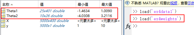
参数矩阵Θ(1) (Theta1) 和 Θ(2) (Theta2) 的维数是如何确定的呢?
一般,对于一个特定的训练数据集而言,它的输入维数 和输出的结果数目是确定的。比如,本文中的数字图片是用一个400维的特征向量代表,输出结果则是0-9的阿拉伯数字,即一共有10种输出。而中间隐藏层的个数则是变化的,根据实际情况选择隐藏层的数目。本文中隐藏层单元个数为25个。故参数矩阵Θ(1) (Theta1)是一个25*401矩阵,行的数目为25,由隐藏层的单元个数决定(不包括bias unit),列的数目由输入特征数目决定(加上bias unit之后变成401)。同理,参数矩阵Θ(2) (Theta2)是一个10*26矩阵,行的数目由输出结果数目决定(0-9 共10种数字),列的数目由隐藏层数目决定(25个隐藏层的unit,再加上一个bias unit)。神经网络的结构图如下:

②代价函数
未考虑正则化的神经网络的代价函数如下:
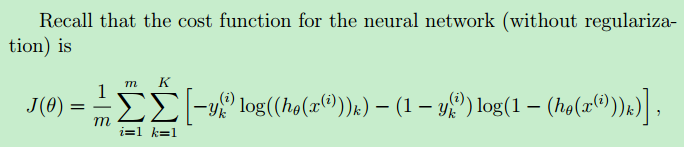
其中,m等于5000,表示一共有5000个训练实例;K=10,总共有10种可能的训练结果(数字0-9)
假设函数 hθ(x(i)) 和 hθ(x(i))k 的解释
我们是通过如下公式来求解hθ(x(i))的:a(1) = x 再加上bias unit a0(1) ,其中,x 是训练集矩阵 X 的第 i 行(第 i 个训练实例)。它是一个400行乘1列的 列向量,上标(1)表示神经网络的第几层。
z(2) = Θ(1) * a(1) ,再使用 sigmoid函数作用于z(2),就得到了a(2),它代表隐藏层的每个神经元的值。a(2)是一个25行1列的列向量。
a(2) = sigmoid(z(2)) ,再将隐藏层的25个神经元,添加一个bias unit ,就a0(2)可以计算第三层(输出层)的神经单元向量a(3)了。a(3)是一个10行1列的列向量。
同理,z(3) = Θ(2) * a(2) , a(3) = sigmoid(z(3)) 此时得到的 a(3) 就是假设函数 hθ(x(i))
由此可以看出:假设函数 hθ(x(i))就是一个10行1列的列向量,而 hθ(x(i))k 就表示列向量中的第 k 个元素。【也即该训练实例以 hθ(x(i))k 的概率取数字k?】
举个例子: hθ(x(6)) = (0, 0, 0.03, 0, 0.97, 0, 0, 0, 0, 0)T 【hθ(x(i))的输出结果是什么,0-1之间的各个元素的取值概率?matlab debug???】
它是含义是:使用神经网络 训练 training set 中的第6个训练实例,得到的训练结果是:以0.03的概率是 数字3,以0.97的概率是 数字5
(注意:向量的下标10 表示 数字0)
训练样本集的 结果向量 y (label of result)的解释
由于神经网络的训练是监督学习,也就是说:样本训练数据集是这样的格式:(x(i), y(i)),对于一个训练实例x(i),我们是已经确定知道了它的正确结果是y(i),而我们的目标是构造一个神经网络模型,训练出来的这个模型的假设函数hθ(x),对于未知的输入数据x(k),能够准确地识别出正确的结果。
因此,训练数据集(traing set)中的结果数据 y 是正确的已知的结果,比如y(600) = (0, 0, 0, 0, 1, 0, 0, 0, 0, 0)T 表示:训练数据集中的第600条训练实例它所对应的正确结果是:数字5 (因为,向量y(600)中的第5个元素为1,其它所有元素为0),另外需要注意的是:当向量y(i) 第10个元素为1时 代表数字0。
③BP(back propagation)算法
BP算法是用来 计算神经网络的代价函数的梯度。
计算梯度,本质上是求偏导数。来求解偏导数我们可以用传统的数学方法:求偏导数的数学计算公式来求解。这也是Ng课程中讲到的“Gradient Checking”所用的方法。但当我们的输入特征非常的多(上百万...),参数矩阵Θ非常大时,就需要大量地进行计算了(Ng在课程中也专门提到,当实际训练神经网络时,要记得关闭 "Gradient Checking")。而这也是神经网络大拿Minsky 曾经的一个观点:(可参考这篇博文:神经网络浅讲)
Minsky认为,如果将计算层增加到两层,计算量则过大,而且没有有效的学习算法。所以,他认为研究更深层的网络是没有价值的。
而BP算法,则解决了这个计算量过大的问题。BP算法又称反向传播算法,它从输出层开始,往输入层方向以“某种形式”的计算,得到一组“数据“,而这组数据刚好就是我们所需要的 梯度。
Once you have computed the gradient, you will be able to train the neural network
by minimizing the cost function J(Θ) using an advanced optimizer such as fmincg.
Sigmoid 函数的导数
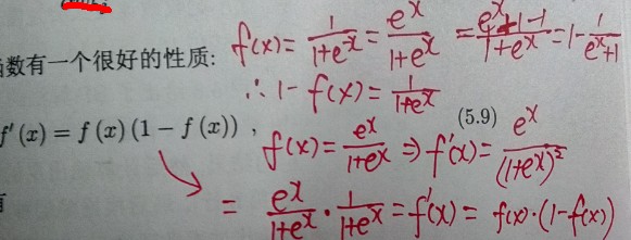
至于为什么要引入Sigmoid函数,等我有了更深刻的理解再来解释(Ng课程中也有提到)。Sigmoid函数的导数有一个特点,即Sigmoid的导数可以用Sigmoid函数自己本身来表示,如下:

证明过程如下:(将 证明过程中的 f(x) 视为 g(z) 即可 )
Sigmoid 函数的Matlab实现如下(sigmoidGradient.m):

g = zeros(size(z));

% ====================== YOUR CODE HERE ======================
% Instructions: Compute the gradient of the sigmoid function evaluated at
%               each value of z (z can be a matrix, vector or scalar).

g = sigmoid(z) .* (1 - sigmoid(z));
% =============================================================
训练神经网络时的“symmetry”现象---随机初始化神经网络的参数矩阵(权值矩阵Θ)
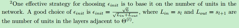
随机初始化参数矩阵,就是对参数矩阵Θ(L)中的每个元素,随机地赋值,取值范围一般为[ξ ,-ξ],ξ 的确定规则如下:
假设将参数矩阵Θ(L) 中所有的元素初始化0,则 根据计算公式:a1(2) = Θ(1) * (参看视频,完善)会导致 a(2) 中的每个元素都会取相同的值。
因此,随机初始化的好处就是:让学习 更有效率
This range of values ensures that the parameters are kept small and makes the learning more efficient
随机初始化的Matlab实现如下:可以看出,它是先调用 randInitializeWeights.m 中定义的公式进行初始化的。然后,再将 initial_Theta1 和 initial_Theta2 unroll 成列向量
initial_Theta1 = randInitializeWeights(input_layer_size, hidden_layer_size);
initial_Theta2 = randInitializeWeights(hidden_layer_size, num_labels);

% Unroll parameters
initial_nn_params = [initial_Theta1(:) ; initial_Theta2(:)];
randInitializeWeights.m 的实现如下:
function W = randInitializeWeights(L_in, L_out)
%RANDINITIALIZEWEIGHTS Randomly initialize the weights of a layer with L_in
%incoming connections and L_out outgoing connections
%   W = RANDINITIALIZEWEIGHTS(L_in, L_out) randomly initializes the weights
%   of a layer with L_in incoming connections and L_out outgoing
%   connections.
%
%   Note that W should be set to a matrix of size(L_out, 1 + L_in) as
%   the column row of W handles the "bias" terms
%
% You need to return the following variables correctly
W = zeros(L_out, 1 + L_in);

% ====================== YOUR CODE HERE ======================
% Instructions: Initialize W randomly so that we break the symmetry while
%               training the neural network.
%
% Note: The first row of W corresponds to the parameters for the bias units
%
epsilon_init = 0.12;
W = rand(L_out, 1 + L_in) * 2 * epsilon_init - epsilon_init;

% =========================================================================

end
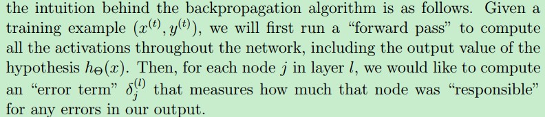
BP算法的具体执行步骤如下:
对于每一个训练实例(x, y),先用“前向传播算法”计算出 activations(a(2), a(3)),然后再对每一层计算一个残差δj(L) (error term)。注意:输入层(input layer)不需要计算残差。
具体的每一层的残差计算公式如下:(本文中的神经网络只有3层,隐藏层的数目为1)
对于输出层的残差计算公式如下,这里的输入层是第1层,隐藏层是第2层,输出层是第3层

残差δ(3)是一个向量,下标 k 表示,该向量中的第 k 个元素。yk 就是前面提到的表示 样本结果的向量y 中的第 k 个元素。(这里的向量 y 是由训练样本集的结果向量y分割得到的)
上面的减法公式用向量表示为:δ(3)= a(3) - y,因此δ(3)维数与a(3)一样,它与分类输出的数目有关。在本例中,是10,故δ(3)是一个10*1向量
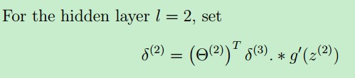
对于隐藏层的残差计算公式如下:
当每一层的残差计算好之后,就可以更新 Δ(delta) 矩阵了,Δ(delta) 矩阵与 参数矩阵有相同的维数,初始时Δ(delta) 矩阵中的元素全为0.
% nnCostFunction.m
Theta1_grad = zeros(size(Theta1));% Theta1_grad is a 25*401 matrix--矩阵Θ(1) ,由Δ(1)的值来更新 Theta2_grad = zeros(size(Theta2));% Theta2_grad is a 10*26 matrix--矩阵Θ(2) ,由Δ(2) 的值来更新
它的定义(计算公式)如下:
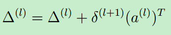
在这里,δ(L+1)是一个列向量,(a(1))T是一个行向量,相乘后,得到的是一个矩阵。
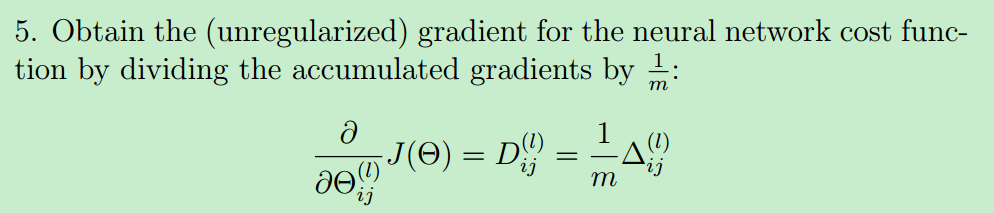
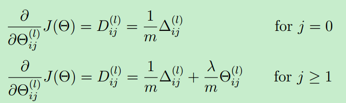
计算出 Δ(delta) 矩阵后,就可以用它来更新 代价函数的导数了,公式如下:
对于一个训练实例(training instance),一次完整的BP算法运行Matlab代码如下:
for i = 1:m
    a1 = X(i, :)'; %the i th input variables, 400*1
    z2 = Theta1 *  a1;
    a2 =  sigmoid( z2 ); % Theta1 * x superscript i
    a2 = [ 1; a2 ];% add bias unit, a2's size is 26 * 1
    z3 = Theta2 * a2;
    a3 = sigmoid( z3 ); % h_theta(x)

    error_3 = a3 - Y( :, i ); % last layer's error, 10*1  第三层的残差计算公式
    %error_2 = ( Theta2' * error_3 ) .*  ( a2 .* (1 - a2) );% g'(z2)=g(z2)*(1-g(z2)), 26*1

    err_2 =  Theta2' * error_3; % 26*1
    error_2 = ( err_2(2:end) ) .*  sigmoidGradient(z2);% 去掉 bias unit 对应的 error units

    Theta2_grad = Theta2_grad + error_3 * a2'; % Δ(L) = Δ(L) + δ(L+1)* (a(L))TTheta1_grad = Theta1_grad + error_2 * a1'; end Theta2_grad = Theta2_grad / m; % video 9-2 backpropagation algorithm the 11 th minute Theta1_grad = Theta1_grad / m; %这里的结果就是 Di,j(L)
④梯度检查(gradient checking)
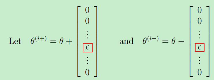
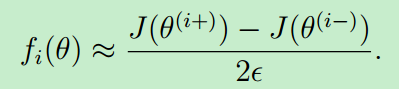
梯度检查的原理如下:由于我们通过BP算法这种巧妙的方式求得了代价函数的导数,那它到底正不正确呢?这里就可以用 高等数学 里面的导数的定义(极限的定义)来计算导数,然后再比较:用BP算法求得的导数 和 用导数的定义 求得的导数 这二者之间的差距。
导数定义(极限定义)---非正式定义,如下:
可能正是这种通过定义直接计算的方式 运算量很大,所以课程视频中才提到:在正式训练时,要记得关闭 gradient checking
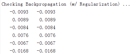
从下面的 gradient checking 结果可以看出(二者计算出来的结果几乎相等),故 BP算法的运行是正常的。
⑤神经网络的正则化
对于神经网络而言,它的表达能力很强,容易出现 overfitting problem,故一般需要正则化。正则化就是加上一个正则化项,就可以了。注意 bias unit不需要正则化
在lambda==1,训练的迭代次数MaxIter==50的情况下,训练的结果如下:代价从一开始的3.29...到最后的 0.52....
训练集上的精度:Training Set Accuracy: 94.820000
Training Neural Network...
Iteration     1 | Cost: 3.295180e+00
Iteration     2 | Cost: 3.250966e+00
Iteration     3 | Cost: 3.216955e+00
Iteration     4 | Cost: 2.884544e+00
Iteration     5 | Cost: 2.746602e+00
Iteration     6 | Cost: 2.429900e+00
.....
.....
.....
Iteration    46 | Cost: 5.428769e-01
Iteration    47 | Cost: 5.363841e-01
Iteration    48 | Cost: 5.332370e-01
Iteration    49 | Cost: 5.302586e-01
Iteration    50 | Cost: 5.202410e-01
对于神经网络而言,很容易产生过拟合的现象,比如当把参数 lambda 设置成 0.1,并且训练次数MaxIter 设置成 200时,训练结果如下:训练精度已经达到了99.94%,很可能是 overfitting 了
Training Neural Network...
Iteration     1 | Cost: 3.303119e+00
Iteration     2 | Cost: 3.241696e+00
Iteration     3 | Cost: 3.220572e+00
Iteration     4 | Cost: 2.637648e+00
Iteration     5 | Cost: 2.182911e+00
....
......
.........
Iteration   197 | Cost: 8.177972e-02
Iteration   198 | Cost: 8.171843e-02
Iteration   199 | Cost: 8.169971e-02
Iteration   200 | Cost: 8.165209e-02

Training Set Accuracy: 99.940000
⑥使用Matlab的 fmincg 函数 最终得到 参数矩阵Θ

% Create "short hand" for the cost function to be minimized
costFunction = @(p) nnCostFunction(p, ...
                                   input_layer_size, ...
                                   hidden_layer_size, ...
                                   num_labels, X, y, lambda);

% Now, costFunction is a function that takes in only one argument (the
% neural network parameters)
[nn_params, cost] = fmincg(costFunction, initial_nn_params, options);
代码中最后一行 fmincg(costFunction, initial_nn_params, options) 将求得的神经网络的参数nn_params返回。initial_nn_params 就上前面提到的使用随机初始化后初始化的参数矩阵。
整个求解代价函数、梯度、正则化的 Matlab代码如下:nnCostFunction.m文件
function [J grad] = nnCostFunction(nn_params, ...
                                   input_layer_size, ...
                                   hidden_layer_size, ...
                                   num_labels, ...
                                   X, y, lambda)
%NNCOSTFUNCTION Implements the neural network cost function for a two layer
%neural network which performs classification
%   [J grad] = NNCOSTFUNCTON(nn_params, hidden_layer_size, num_labels, ...
%   X, y, lambda) computes the cost and gradient of the neural network. The
%   parameters for the neural network are "unrolled" into the vector
%   nn_params and need to be converted back into the weight matrices.
%
%   The returned parameter grad should be a "unrolled" vector of the
%   partial derivatives of the neural network.
%

% Reshape nn_params back into the parameters Theta1 and Theta2, the weight matrices
% for our 2 layer neural network
Theta1 = reshape(nn_params(1:hidden_layer_size * (input_layer_size + 1)), ...
                 hidden_layer_size, (input_layer_size + 1));

Theta2 = reshape(nn_params((1 + (hidden_layer_size * (input_layer_size + 1))):end), ...
                 num_labels, (hidden_layer_size + 1));

% Setup some useful variables
m = size(X, 1);

% You need to return the following variables correctly
J = 0;
Theta1_grad = zeros(size(Theta1));% Theta1_grad is a 25*401 matrix
Theta2_grad = zeros(size(Theta2));% Theta2_grad is a 10*26 matrix

% ====================== YOUR CODE HERE ======================
% Instructions: You should complete the code by working through the
%               following parts.
%
% Part 1: Feedforward the neural network and return the cost in the
%         variable J. After implementing Part 1, you can verify that your
%         cost function computation is correct by verifying the cost
%         computed in ex4.m
X = [ones(m,1) X]; %5000*401
a_super2 = sigmoid(Theta1 * X'); % attention a_super2 is a 25*5000 matrix
a_super2 = [ones(1,m);a_super2]; %add each bias unit for a_superscript2, 26 * 5000

% attention a_super3 is a 10 * 5000 matrix, each column is a predict value
a_super3 = sigmoid(Theta2 * a_super2);%10*5000

a3 = 1 - a_super3;%10*5000

%将5000条的结果label 向量y 转化成元素只为0或1 的矩阵Y
Y = zeros(num_labels, m); %10*5000, each column is a label result
for i = 1:num_labels
    Y(i, y==i)=1;
end

Y1 = 1 - Y;
res1 = 0;
res2 = 0;
for j = 1:m
    %两个矩阵的每一列相乘,再把结果求和。预测值和结果label对应的元素相乘,就是某个输入x 的代价
    tmp1 = sum( log(a_super3(:,j)) .* Y(:,j) );
    res1 = res1 + tmp1; % m 列之和
    tmp2 = sum( log(a3(:,j)) .* Y1(:,j) );
    res2 = res2 + tmp2;
end
J = (-res1 - res2) / m;

%
% Part 2: Implement the backpropagation algorithm to compute the gradients
%         Theta1_grad and Theta2_grad. You should return the partial derivatives of
%         the cost function with respect to Theta1 and Theta2 in Theta1_grad and
%         Theta2_grad, respectively. After implementing Part 2, you can check
%         that your implementation is correct by running checkNNGradients
%
%         Note: The vector y passed into the function is a vector of labels
%               containing values from 1..K. You need to map this vector into a
%               binary vector of 1's and 0's to be used with the neural network
%               cost function.
%
%         Hint: We recommend implementing backpropagation using a for-loop
%               over the training examples if you are implementing it for the
%               first time.
%

for i = 1:m
    a1 = X(i, :)'; %the i th input variables, 400*1
    z2 = Theta1 *  a1;
    a2 =  sigmoid( z2 ); % Theta1 * x superscript i
    a2 = [ 1; a2 ];% add bias unit, a2's size is 26 * 1
    z3 = Theta2 * a2;
    a3 = sigmoid( z3 ); % h_theta(x)

    error_3 = a3 - Y( :, i ); % last layer's error, 10*1
    %error_2 = ( Theta2' * error_3 ) .*  ( a2 .* (1 - a2) );% g'(z2)=g(z2)*(1-g(z2)), 26*1

    err_2 =  Theta2' * error_3; % 26*1
    error_2 = ( err_2(2:end) ) .*  sigmoidGradient(z2);% 去掉 bias unit 对应的 error units

    Theta2_grad = Theta2_grad + error_3 * a2';
    Theta1_grad = Theta1_grad + error_2 * a1';
end

Theta2_grad = Theta2_grad / m; % video 9-2 backpropagation algorithm the 11 th minute
Theta1_grad = Theta1_grad / m;

% Part 3: Implement regularization with the cost function and gradients.
%
%         Hint: You can implement this around the code for
%               backpropagation. That is, you can compute the gradients for
%               the regularization separately and then add them to Theta1_grad
%               and Theta2_grad from Part 2.
%

% reg for cost function J,  ex4.pdf page 6
Theta1_tmp = Theta1(:, 2:end).^2;
Theta2_tmp = Theta2(:, 2:end).^2;
reg = lambda / (2*m) * ( sum( Theta1_tmp(:) ) + sum( Theta2_tmp(:) ) );

J = (-res1 - res2) / m + reg;
% -------------------------------------------------------------

% reg for bp, ex4.pdf materials page 11
Theta1(:,1) = 0;
Theta2(:,1) = 0;

Theta1_grad = Theta1_grad + lambda / m * Theta1;
Theta2_grad = Theta2_grad + lambda / m * Theta2;
% =========================================================================

% Unroll gradients
grad = [Theta1_grad(:) ; Theta2_grad(:)];
end
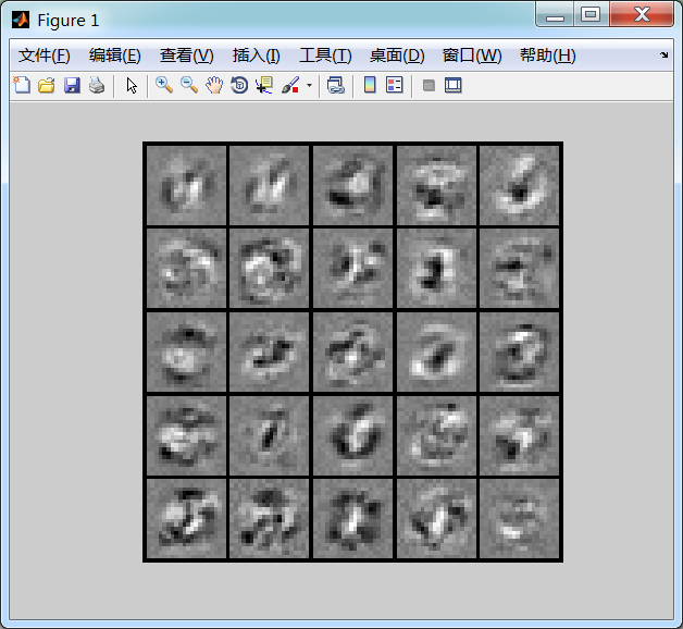
⑦可视化神经网络
多层神经网络有很多层,层数越多,有着更深的表示特征及更强的函数模拟能力。后一层网络是前一层的更“抽象”(更深入)的表示。
比如说本文中的识别0-9数字,这里的隐藏层只有一层(一般而言第一层称为输入层,最后一层称为输出层,其他中间的所有层称为隐藏层),隐藏层它学到的只是数字的一些边缘特征,输出层在隐藏层的基础上,就基本上能识别数字了。
隐藏层的可视化如下:
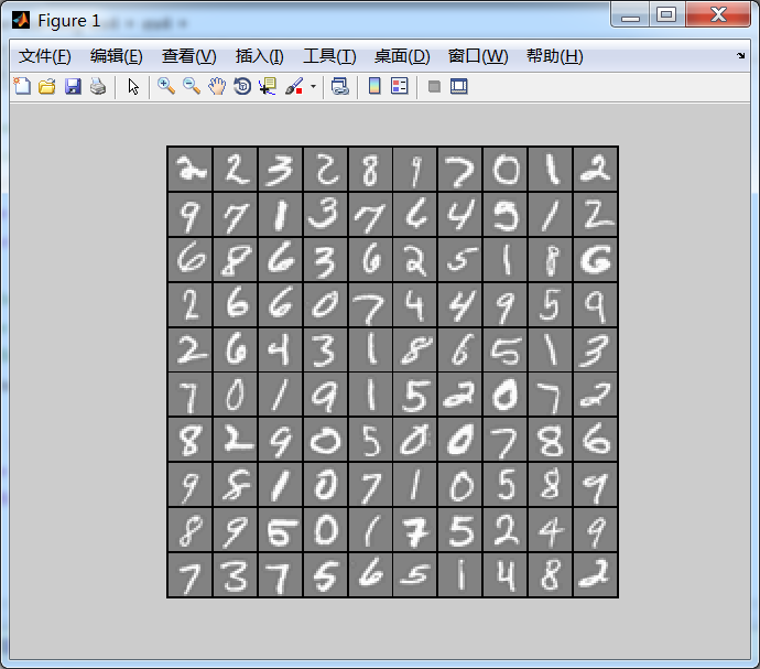
输出层的可视化 “可能”如下:
原文:http://www.cnblogs.com/hapjin/p/6106182.html